
views
- On desktop, click the column letter to highlight it. Right-click, then click "Conditional formatting". Apply a color, then click "Done".
- On Android, tap the column letter, then the "A" icon. Tap "Conditional formatting". Apply a color, then tap "Done".
- On iOS, tap the column letter. Tap the "A" icon. Tap "Cell", then select a Fill color.
Using Desktop

Open a spreadsheet in Google Sheets on your web browser. This can be a new or existing spreadsheet. You can use Google Chrome, Safari, Mozilla Firefox, or another browser. You will need a Google account to use Google Sheets. If you aren't already logged in, enter your login details and click Sign in to do so now.
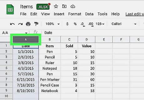
Highlight the column you want to color. You can do this by clicking the column letter at the top of the spreadsheet. You can also click any cell in the column, then press CTRL + Space (Windows) or Command + Space (Mac) to highlight the entire column. If needed, you can add another column.
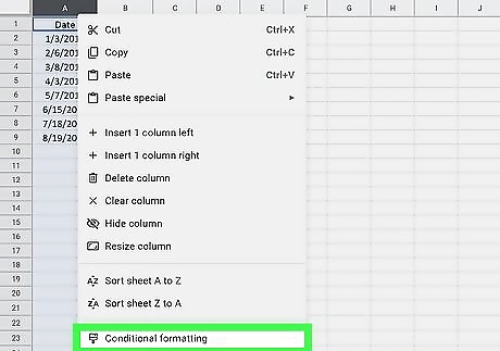
Right-click the column and click Conditional formatting. This will be next to a paintbrush icon. A new panel will open on the right side. You can also click the down-arrow next to the column letter (A, B, C, etc.) or go to Format → Conditional formatting. If you have an existing rule in the spreadsheet, click Add another rule.
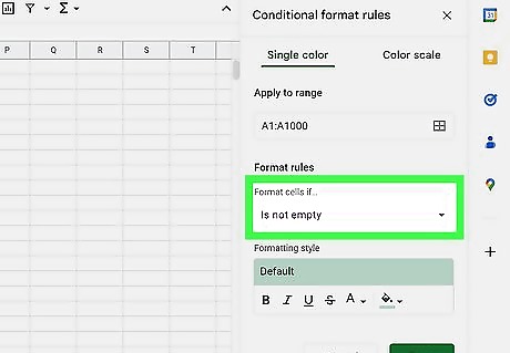
Apply the Format rules. If you want to highlight the text-filled cells, click the drop-down menu under Format cells if… and select Is not empty. If you want to highlight the empty cells, select Is empty. If you want to apply a formula, select Custom formula is at the very bottom of the drop-down menu. Insert the value or formula.
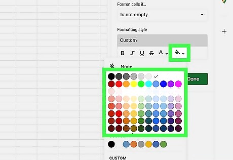
Apply the Formatting style. Click the paint bucket icon to select the highlight color. You can also apply boldness, italics, underline, strikethrough, or change the text color. If you want to choose a Formatting preset, click Default and select the preset.
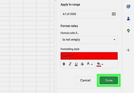
Click Done. This is the green button below the Conditional format rules. Your column will be highlighted. You can also highlight duplicate cells.
Using Android
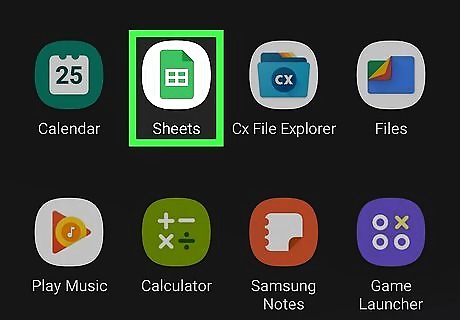
Open the Google Sheets app on your Android device. This looks like a green spreadsheet with a white background. Google Sheets is available for Android in the Google Play Store. You must have a Google account to use Google Sheets. If you don't have an account, you can create one. This method will not work on iOS. You can see conditional formatting rules on an iOS device, but you cannot create or edit them.

Open a new or existing spreadsheet. Scroll through your Recents page and tap an existing spreadsheet or tap the + to create a new one.
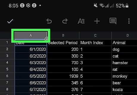
Tap the column letter. This will select the column you want to highlight.
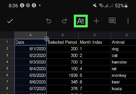
Tap the Format icon. This is the A with lines to its right. You can find this at the top-right corner, next to +.
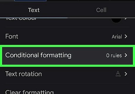
Tap Conditional formatting. This will be between Font and Text rotation. A new panel will open. If you have an existing rule in the spreadsheet, tap ADD first.
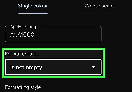
Apply the Format rules. If you want to highlight the text-filled cells, tap the drop-down menu under Format cells if… and select Is not empty. If you want to highlight the empty cells, select Is empty. If you want to apply a formula, select Custom formula is at the very bottom of the drop-down menu. Insert the value or formula.
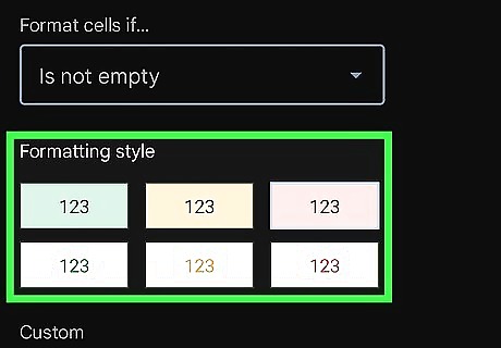
Apply the Formatting style. You can select from the presets, or tap + to create a custom style. When creating a custom style, you can apply boldness, italics, underline, strikethrough, change the highlight color, or change the text color. To change the highlight color, tap the paint bucket icon and select the color.
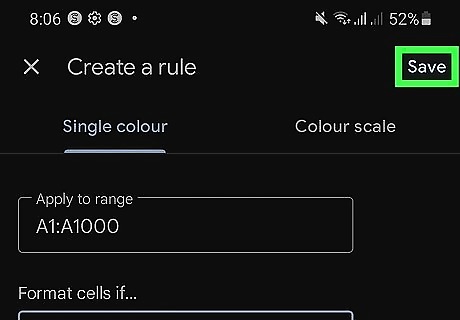
Tap Save. This will be at the top-right corner. Your column will be highlighted.
Using iPhone or iPad

Open the Google Sheets app on your iPhone or iPad. This looks like a green spreadsheet with a white background. Google Sheets is available for iOS in the App Store. If you aren't already logged in to your Google account, enter your login details and click Sign in to do so now. This method involves changing the cell color of a column without the use of conditional formatting rules.

Open a new or existing spreadsheet. Scroll through your Recents page and tap an existing spreadsheet or tap the + to create a new one.
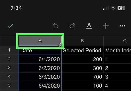
Tap the column letter. This will select the column you want to highlight.
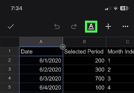
Tap the Format icon. This is the underlined A. You can find this at the top-right corner, next to +. A pop-up menu will open.
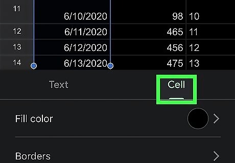
Tap the "Cell" tab. This is to the right of the Text tab.
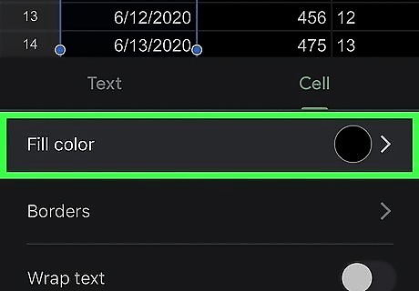
Tap Fill color. By default, the Fill color will be white.
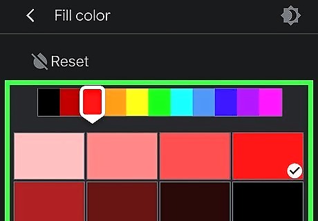
Select a color. Tap a main color in the top row to see different shades. Toggle brightness with the sun icon in the top-right corner of the Fill color menu. The color will be applied immediately.
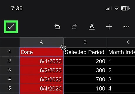
Tap the check mark icon to save. This will be in the top-left corner of the spreadsheet.


Comments
0 comment