views
- Go to Formulas > AutoSum to automatically add up a column.
- Use the SUM function to add individual or multiple columns.
- To add multiple columns, select the cell range containing each column you want to sum.
Using AutoSum for One Column
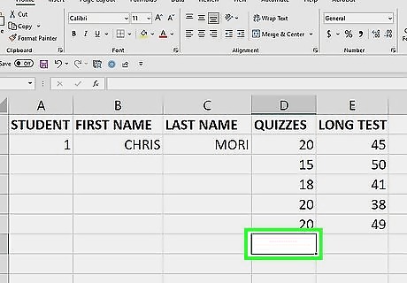
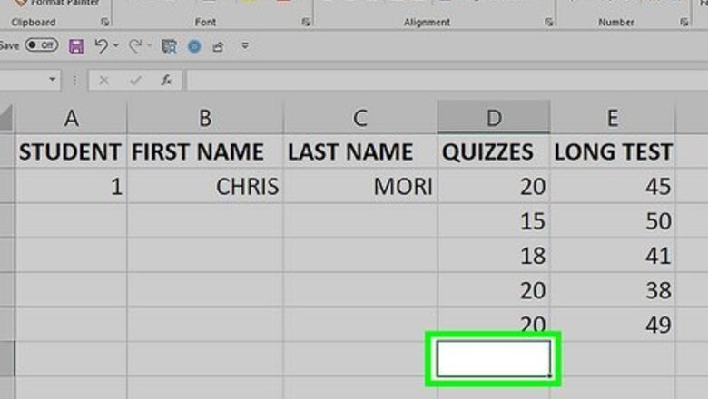
Click the cell directly below the values you want to sum. For example, if you have values in cells A1 through A5, you would click A6. If you’re just getting started with Excel, check out our intro guides for making a spreadsheet and formatting a spreadsheet.
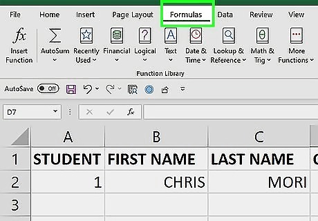
Click the Formulas tab. This will display various formula options in the top bar.
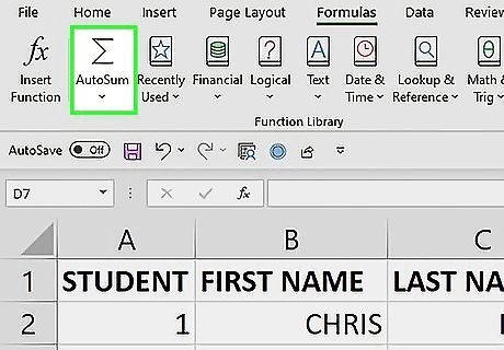
Click AutoSum. This will open a drop down menu with AutoSum options.
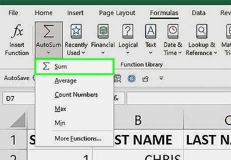
Click Sum. This will automatically create a SUM function that adds the values of the column. You’ll see the values that are going to be summed in a highlighted selection box.

Press ↵ Enter or ⏎ Return on your keyboard. This will confirm the SUM formula and show you the sum total in the cell you selected.
Using SUM for One Column
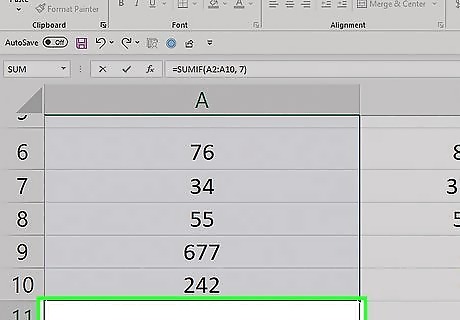
Click a cell below the column you want to add up. Doing so will place your cursor in the cell. This method uses the SUM function, which adds all of the values in a given cell range. If you’re looking for subtraction information, check out our guide to subtracting in Excel.
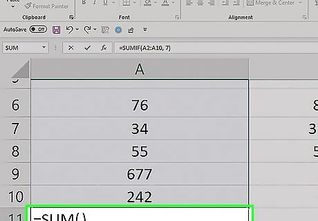
Enter the "SUM" function. Type =SUM() into the cell.
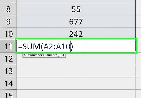
Enter the column's range. Type the top cell in the column, a colon, and the bottom cell in the column into the parentheses. For example, if you're adding values in the A column and you have data in cells A2 through A10, you would type in the following: =SUM(A2:A10) If your dataset has a header row, don’t include the header in the SUM formula.

Press ↵ Enter or ⏎ Return. This will display the sum of the column in your selected cell.
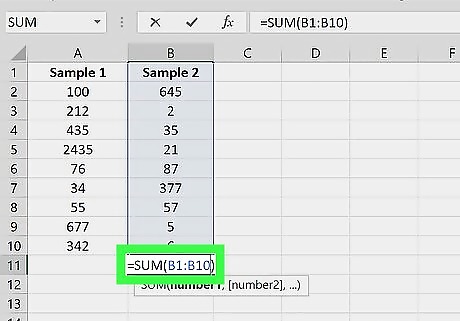
Create the sums of the other columns you want to add. You can create SUM formulas for each column, or copy the first formula: To quickly sum other columns of the same length, you can press Ctrl+c (Windows) to copy the cell with the SUM formula, then press Ctrl+v (Windows) to paste it under the other columns. On Mac, these shortcuts are ⌘ Cmd+c and ⌘ Cmd+v respectively. Pasting the formula will automatically change the cell references to the column that corresponds with where you pasted the formula.
Using SUM for Multiple Columns
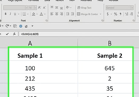
Determine which of your columns is the longest. This method adds up multiple columns in one formula. In order to include all of the cells in the longest column, you'll need to know to which row the column extends. For example, if you have three columns and the longest one has values from row 1 through row 20, your formula will need to include rows 1 through 20 for each column you want to add even if this includes blank cells.
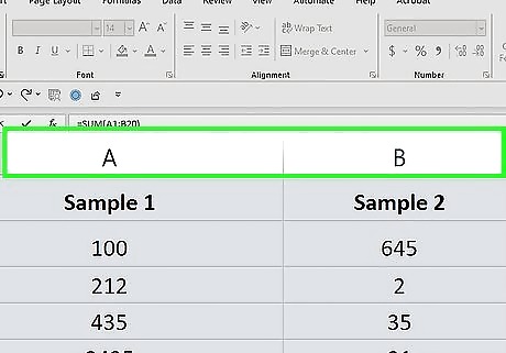
Determine your beginning and ending columns. If you're adding the A column and the B column, for example, your beginning column is the A column and your ending column is the B column.
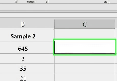
Select a blank cell. Click the cell in which you want to display the sum of your columns.
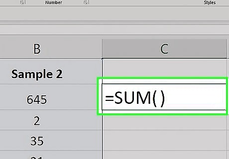
Enter the "SUM" command. Type =SUM() into the cell.
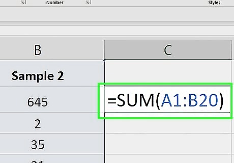
Enter the cell range. For a range of cells, the left cell in the range is the top-left cell, and the right cell is the bottom-right cell. These two cells define the range. In other words, type the first column letter, the first row number, a colon, the last column letter, and the last row number. For example, if you're adding columns A, B, and C, and your longest column stretches to row 20, you would enter the following: =SUM(A1:C20)

Press ↵ Enter or ⏎ Return. Doing so will display the sum of all of the columns in your selected cell.
Using SUMIF
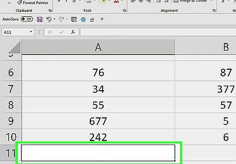
Click a cell below the column you want to add up. Doing so will place your cursor in the cell. This method uses the SUMIF function, which allows you to add values in a data range if they meet a certain criteria.
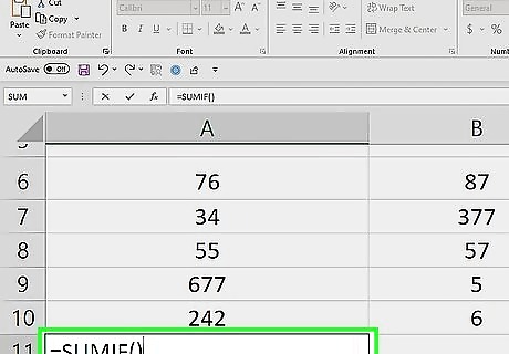
Enter the "SUMIF" function. Type =SUMIF() into the cell. SUMIF has three arguments: range, criteria, [sum_range]. The [sum_range] argument is optional and used to specify a different range to sum values in. The criteria argument will check the range specified in the first argument.
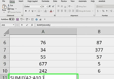
Enter the column's range and a comma. Type the top cell in the column, a colon, and the bottom cell in the column into the parentheses. For example, if you're checking the values in the A column and you have data in cells A2 through A10, you would type in the following: =SUMIF(A2:A10,) If your dataset has a header row, don’t include the header in the SUM formula.
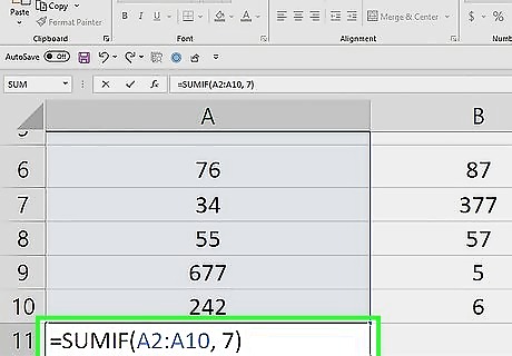
Enter the criteria you want to check. Place the criteria as the second argument after the comma. This can be a cell reference, text, number, expression, or function. Each cell in the specified range will be checked using this criteria. If the criteria is met, it will be added to the total sum. Here are a few examples: =SUMIF(A2:A10, 7) would check whether a value equals 7. =SUMIF(A2:A10, "<10") would check whether a value is less than 10. Note that logical criteria needs quotation marks. =SUMIF(A2:A10, "cat") would check whether the value is the word "cat".
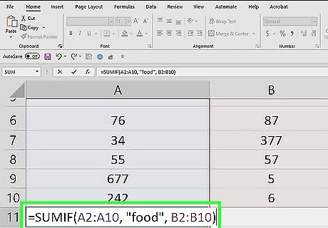
Enter a comma and a sum range (optional). Place a comma after the criteria argument, then type a sum range. The sum range needs to be the same shape and size as the range in the first argument. SUMIF will check the criteria in the range and add the corresponding value in the sum range. For example, if you had 9 purchases in A2:A10 and their corresponding prices in B2:B10, you could sum the prices of purchase called "food" using this formula: =SUMIF(A2:A10, "food", B2:B10)

Press ↵ Enter or ⏎ Return. This will display the sum in your selected cell.
Using the Status Bar
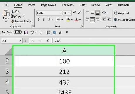
Click a column letter to see the sum of its values. This is the letter header located above the spreadsheet cells. The entire column will be highlighted.
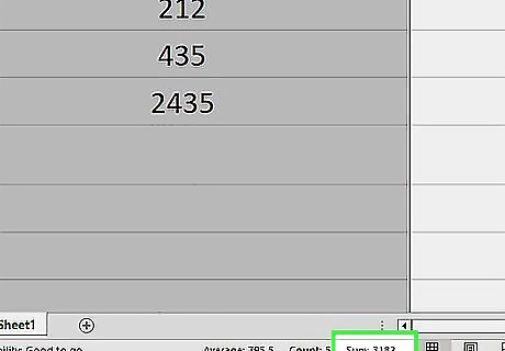
Look at the status bar to see the sum. At the bottom of Excel is the status bar. The sum total of the values in the column will be displayed next to "sum:".
Using a Table
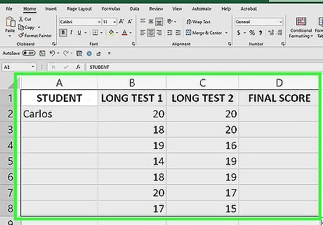
Select your dataset. Click and drag from the top left to the bottom right of your dataset to select it. This method changes the dataset into a table, to which you can add a total row.

Click the Home tab. It's at the top of the Excel window.
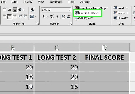
Click Format as Table. A drop down menu will appear with table options.
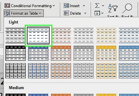
Select a table style. You can select from a variety of colors and formats. A small window titled "Create table" will appear after selecting a style.
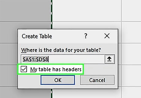
Check the box next to "My table has headers" (if needed). If your dataset has a header row, select this option to format the table correctly. Otherwise, uncheck the box.
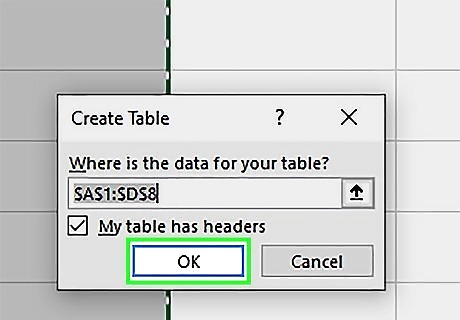
Click OK. This will change the dataset into a table.
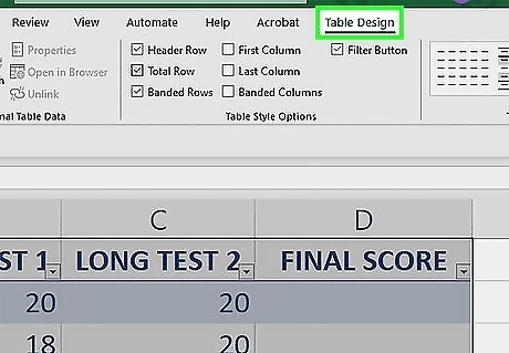
Click the Table Design tab. It's at the top of the Excel window.
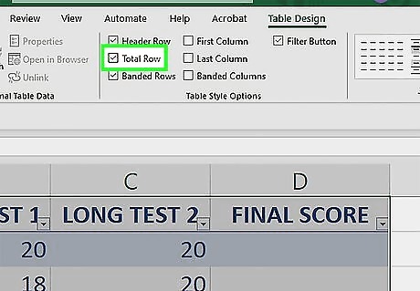
Check the box next to "Total Row". This is an option in the "Table Style Options" section of the Table Design tab.
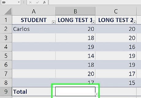
Click the cell in the total row in the column you want to sum. A drop down arrow will appear next to the cell. For example, if your data is in A2:A10 and the total row is in row 11, you would click A11.
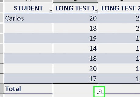
Click the drop down arrow ▼. This will display a down down menu with total options.
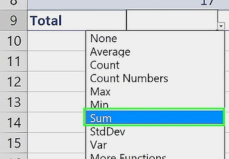
Select Sum. This is an option in the total drop down menu. A sum total for that column will appear in the cell. You're done!


Comments
0 comment