views
- Calculate the coefficient by finding Σd2, then plugging that value into the Spearman's rank correlation coefficient formula.
- You can also easily calculate this coefficient using Excel.
- Alternatively, you can find this coefficient using R commands.
By Hand

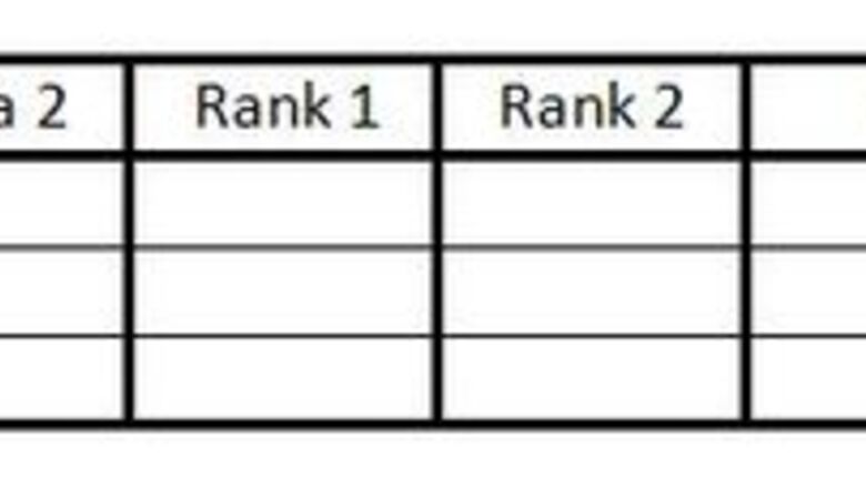
Draw your data table. This will organize the information you need to calculate Spearman's Rank Correlation Coefficient. You will need: 6 Columns, with headers as shown below. As many rows as you have pairs of data.

Fill in the first two columns with your pairs of data.

In your third column rank the data in your first column from 1 to n (the number of data you have). Give the lowest number a rank of 1, the next lowest number a rank of 2, and so on.

In your fourth column do the same as in step 3, but instead rank the second column. Mean_742.jpgIf two (or more) pieces of data in one column are the same, find the mean of the ranks as if those pieces of data had been ranked normally, then rank the data with this mean. In the example at right, there are two 5s that would otherwise have ranks of 2 and 3. Since there are two 5s, take the mean of their ranks. The mean of 2 and 3 is 2.5, so assign the rank 2.5 to both 5s.

In the "d" column calculate the difference between the two numbers in each pair of ranks. That is, if one is ranked 1 and the other 3 the difference would be 2. (The sign doesn't matter, since the next step is to square this number.)

Square each of the numbers in the "d" column and write these values in the "d" column.

Add up all the data in the "d" column. This value is Σd.Step7_812.jpg

Choose one of these formulae: If there was no tie in previous steps, insert this value into the simplified Spearman's Rank Correlation Coefficient formulaStep8_271.jpg and replace the "n" with the number of pairs of data you have to calculate the answer. Step9_402.jpg If there were ties in any of previous steps, use the standard Spearman's Rank Correlation Coefficient formula instead:Spearman.png
Interpret your result. It can vary between -1 and 1. Close to -1 - Negative correlation. Close to 0 - No linear correlation. Close to 1 - Positive correlation.
In Excel
Create new columns with the ranks of your existing columns. For example, if your data is in Column A2:A11, you want to use the formula "=RANK(A2,A$2:A$11)", and copy it down and across for all your rows and columns.
Break ties as described in step 3, 4 method 1.
In a new cell, do a correlation between the two rank columns with something like "=CORREL(C2:C11,D2:D11)". In this case, C and D would correspond to the rank columns. The correlation cell will have your Spearman's Rank Correlation.
Using R
Get R if you don't already have it. (See http://www.r-project.org.)
Save your data as a CSV file with the data you want to correlate in the first two columns. You can typically do this through the "Save as" menu.
Open the R editor. If you are on the terminal, simply run R. From the desktop, you want to click on the R logo.
Type the commands: d <- read.csv("NAME_OF_YOUR_CSV.csv") and hit enter cor(rank(d[,1]),rank(d[,2]))


Comments
0 comment