How to Delete a Pivot Table

• To delete an entire Pivot Table quickly, click anywhere in the table, press Cmd + A (Mac) or Ctrl + A (PC), and then press the Delete key.
• If you want to keep the calculations from your Pivot Table but remove the table formatting, you can copy the data and paste it using Paste Values.
• If you get the error "Cannot change this part of a PivotTable report," click the table, go to PivotTable Analyze > Select > Entire PivotTable, then press Delete.

Delete the Pivot Table and All Data

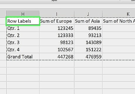
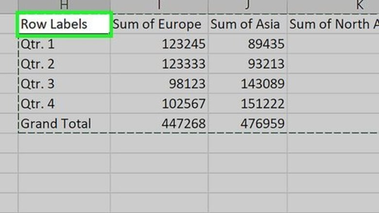
Select the entire Pivot Table. If you want to delete your Pivot Table and all of its calculations, start by clicking and dragging your mouse over the entire table to select it. You can also click anywhere inside of the table and press Ctrl + A (PC) or Cmd + A (Mac) to instantly select the whole table. If you see an error that says "Cannot change this part of a PivotTable report" or it isn't obvious where your Pivot Table ends or begins, there's another simple way to select the table: Click once anywhere in the table. Click the PivotTable Analyze tab (or Analyze tab in some versions). Click Select on the toolbar. Click Entire PivotTable.

Press the Del or Delete key. This instantly deletes the entire Pivot Table from your workbook. Deleting a Pivot Table won't impact the source data used to create the Pivot Table—you'll only be deleting the contents of the table. If your Pivot Table is on its own sheet, you can also simply delete the sheet. To do so, just right-click the sheet's name at the bottom of your workbook and select Delete.

Delete the Table but Keep the Data

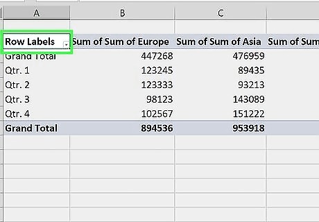
Click any cell in the Pivot Table. If you want to keep the data from your Pivot Table but get rid of the Pivot Table itself, you can convert the table to values. Start by clicking any cell in the table. Use this method if you created a Pivot Table to perform calculations but now want to work with the data as plain, easy-to-edit text.

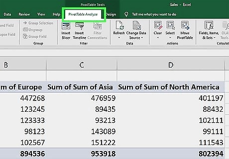
Click the PivotTable Analyze tab. You'll see this at the top of Excel. Depending on your version of Excel, you might see a "PivotTable Tools" tab with a separate Analyze tab on it. If so, click the Analyze tab.

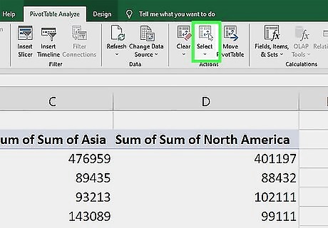
Click Select on the toolbar. A menu will expand.

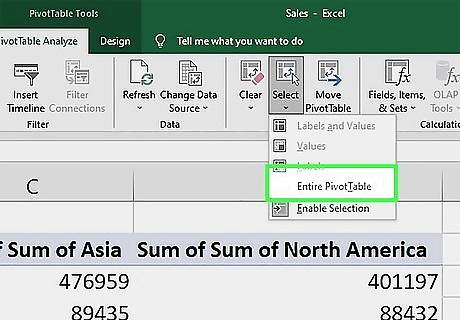
Click Entire PivotTable. This selects the entire table, including any data that is filtered out of view.

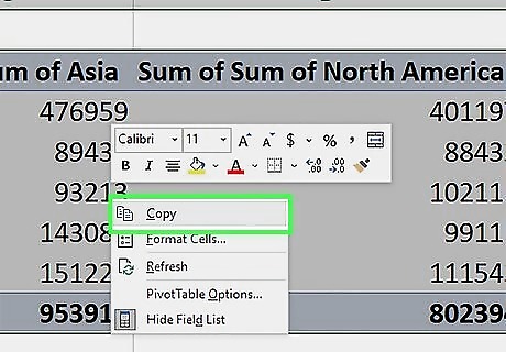
Right-click the Pivot Table and select Copy. The data is now copied to your clipboard.

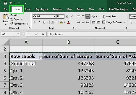
Click the Home tab. It's at the top-left corner of Excel.

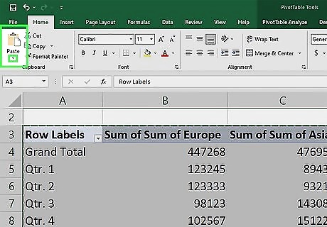
Click the down-arrow below the "Paste" option. You'll see this arrow in the upper-left corner of Excel, below the clipboard icon. Don't click the clipboard icon, as you'll get an error. You have to click that arrow just below the icon.

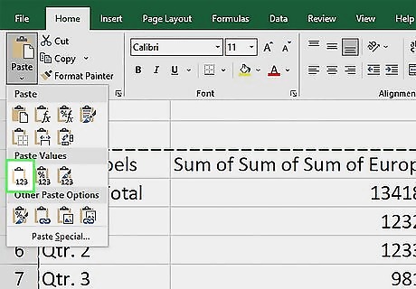
Click the first icon under "Paste Values." It's the small clipboard icon with "123" at the bottom. This replaces the Pivot Table with the selected data. Now that you've removed the PivotTable formatting, you can edit the data as needed.