Simple Steps to Make Tables in Excel

Creating a Table

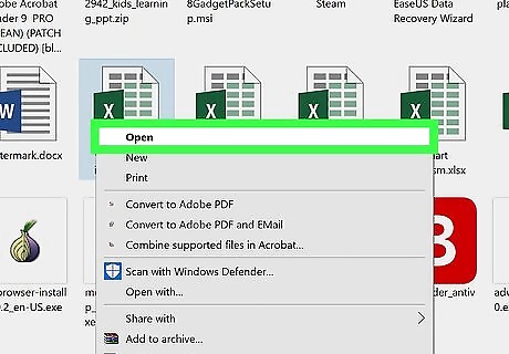
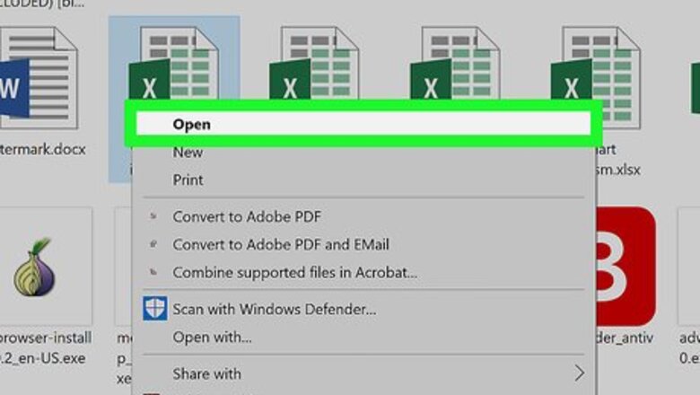
Open your Excel document. Double-click the Excel document, or double-click the Excel icon and then select the document's name from the home page. You can also open a new Excel document by clicking Blank Workbook on the Excel home page, but you'll need to input your data before continuing.

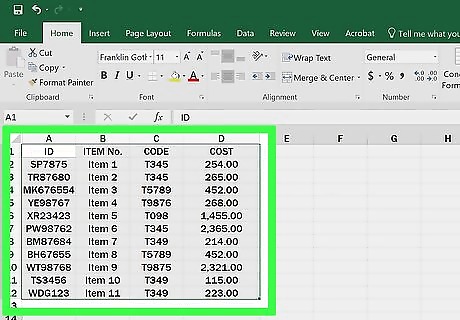
Select your table's data. Click the cell in the top-left corner of the data group you want to include in your table, then hold down ⇧ Shift while clicking the bottom-right cell in the data group. For example: if you have data in cells A1 down to A5 and over to D5, you would click A1 and then click D5 while holding ⇧ Shift.

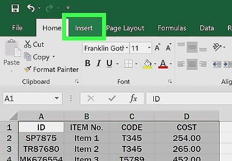
Click the Insert tab. It's a tab in the green ribbon at the top of the Excel window. Doing so will display the Insert toolbar below the green ribbon. If you're on a Mac, make sure you don't click the Insert menu item in your Mac's menu bar.

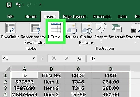
Click Table. This option is in the "Tables" section of the toolbar. Clicking it brings up a pop-up window.

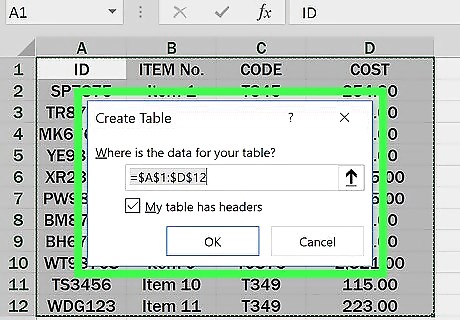
Click OK. It's at the bottom of the pop-up window. Doing so will create your table. If your data group has cells at the top of it that are dedicated to column names (e.g., headers), click the "My table has headers" checkbox before you click OK.

Changing the Table's Design

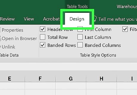
Click the Design tab. It's in the green ribbon near the top of the Excel window. This will open a toolbar for your table's design directly below the green ribbon. If you don't see this tab, click your table to prompt it to appear.

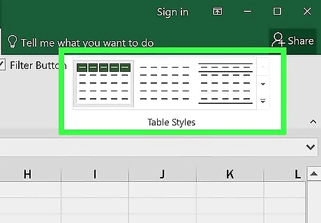
Select a design scheme. Click one of the colored boxes in the "Table Styles" section of the Design toolbar to apply the color and design to your table. You can click the downward-facing arrow to the right of the colored boxes to scroll through different design options.

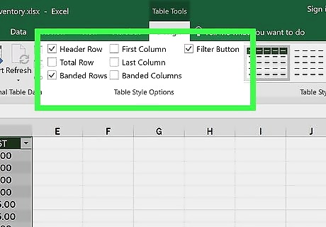
Review the other design options. In the "Table Style Options" section of the toolbar, check or uncheck any of the following boxes: Header Row - Checking this box places column names in the top cell of the data group. Uncheck this box to remove headers. Total Row - When enabled, this option adds a row at the bottom of the table that displays the total value of the right-most column. Banded Rows - Check this box to color in alternating rows, or uncheck it to leave all rows in your table the same color. First Column and Last Column - When enabled, these options make the headers and data in the first and/or last columns bold. Banded Columns - Check this box to color in alternating columns, or uncheck it to leave all columns in your table the same color. Filter Button - When checked, this box places a drop-down box next to each header in your table that allows you to change the data displayed in that column.

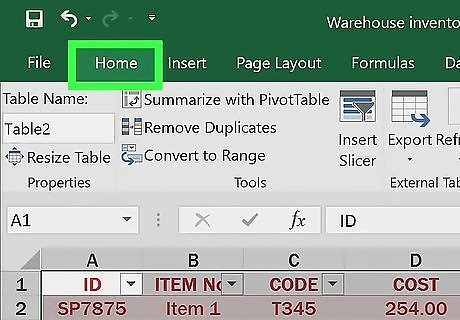
Click the Home tab again. This will take you back to the Home toolbar. Your table's changes will remain.

Filtering Table Data

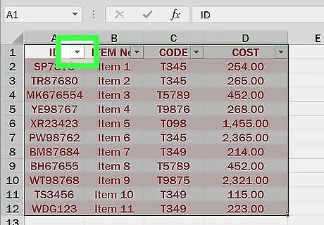
Open the filter menu. Click the drop-down arrow to the right of the header for the column whose data you want to filter. A drop-down menu will appear. In order to do this, you must have both the "Header Row" and the "Filter" boxes checked in the "Table Style Options" section of the Design tab.

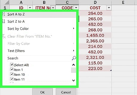
Select a filter. Click one of the following options in the drop-down menu: Sort Smallest to Largest Sort Largest to Smallest You may also have additional options such as Sort by Color or Number Filters depending on your data. If so, you can select one of these options and then click a filter in the pop-out menu.

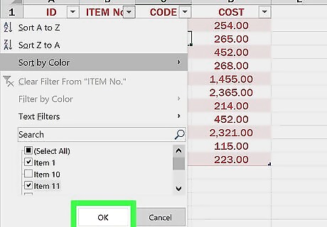
Click OK if prompted. Depending on the filter you choose, you may also have to select a range or a different type of data before you can continue. Your filter will be applied to your table.