
- INDEX retrieves the value of a given location in a range of cells, and MATCH finds the position of an item in a range of cells.
- In an INDEX MATCH function, nested MATCH functions find the row and column numbers for the INDEX function.
- INDEX MATCH outweighs VLOOKUP for a few reasons, the biggest being it can look to columns on the left.
INDEX Function
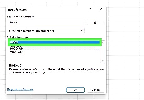
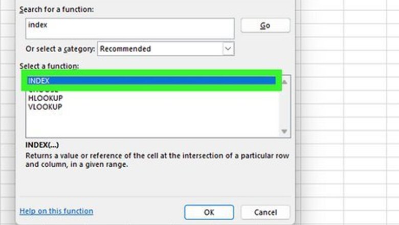
INDEX retrieves the value of a given location in a range. While this might seem rather straightforward, INDEX is a very versatile function that you can use in many ways, some of which are detailed later in this article. There are two ways to use INDEX: the array form and the reference form.

Array form will return the value of an element in a table or array. The syntax for the array form of INDEX is =INDEX(array, row_number, [column_number]). There are three arguments in the array form: array: A range of cells or an array constant. This is a required argument for the function. row_number: Selects the row in an array that you want to return a value from. Must point to a cell within the array or Excel will give you an error. Required, unless you have column_number. column_number: Selects the column in an array that you want to return a value from. Optional. If you're using this argument, it must point to a cell within the array, or Excel will give you an error.
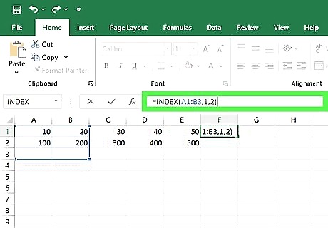
Fill in your variables. For example, if you have a table with two columns and three rows that spans A1 to B3, and you want to return the value at the intersection of the first row and the second column, you would write =INDEX(A1:B3,1,2). If you are omitting either the row number or the column number, you must leave a space for it. Returning the values from the second row of the array would look like =INDEX(A1:B3,2,), and returning the values from the second column of the array would look like =INDEX(A1:B3,,2).

Reference form will return the reference at the intersection of a row and column. The syntax for the array form of INDEX is =INDEX(reference, row_number, [column_number], [area_number]). There are four arguments in the reference form: reference: A reference to one or more cell ranges. This is a required argument for the function. row_number: The number of the row in the reference from which you want to reference. Required. column_number: The column number in the reference from which you want to reference. Optional. area_number: Selects one of your reference ranges from which to return the reference. The first area entered is 1, the second is 2, etc. This is optional, but if you omit it, INDEX will use area one by default. These ranges must also all be on one sheet.
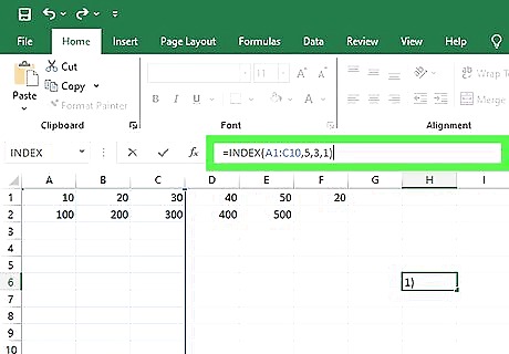
Fill in your variables. For example, if you have a table with three columns and ten rows that spans A1 to C10 and you want to return the value at the intersection of the fifth row and the third column, you would write =INDEX(A1:C10,5,3,1). If you have two reference areas (A1:C3 and A7:C10) and you want to reference a cell that intersects the second row and third column, you would write =INDEX((A1:C3, A7:C10),2,3,1), ensuring that you mark your area number as 1, as that range holds the cell you're trying to reference. If you are omitting either the row number, column number, or area number, you must leave a space for it. If you're referencing the first reference area, like in the example, you could leave the area number out because it defaults to one. As such, your function would look like =INDEX((A1:C3, A7:C10),2,3,).
MATCH Function

MATCH will find the position of an item in a range. MATCH is a very straightforward function: it will simply look for an item in a range that you specify. While MATCH is simple on its own, you can combine it with INDEX—but it's important to understand how MATCH works before using it in conjunction with other functions.

The MATCH function uses three arguments. MATCH's syntax is =MATCH("lookup_value",lookup_array,[match_type]), and the arguments are as follows: lookup_value: The value you want to find in your specified range of cells. The lookup_value can be a value (number, text, or logical) or a cell reference to a number, text, or logical value. Required. lookup_array: The range of cells you want to search. Required. match_type: There are three match types represented by 1, 0, or -1. A match_type of 1 means that MATCH finds the largest value that is less than or equal to the lookup_value. A match_type of 0 means that MATCH finds a value that is exactly equal to the lookup_value. A match_type of -1 means that MATCH finds the smallest value that is greater than or equal to the lookup_value. This value is optional, but if you omit it, the function will default to a match_type of 1.
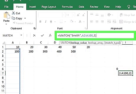
Fill in your variables. If you're trying to find every instance of the last name "Smith" in a cell range from A2 to A100, you would enter =MATCH("Smith",A2:A100,2). You could also leave off the match type in this example, as you get the same result without one—which would leave your function looking like =MATCH("Smith",A2:A100,).
INDEX and MATCH Two-Way Lookup

Combine INDEX and MATCH to create dynamic lookup formulas. INDEX will find the lookup value via row and column numbers, and MATCH will provide the column and row numbers. To make a truly dynamic lookup function, you must nest two MATCH functions inside your INDEX function. The syntax is as follows: =INDEX(array, MATCH("lookup_value", lookup_array, [match_type]), MATCH("lookup_value", lookup_array, [match_type])). Recall back to the original INDEX syntax—your two nested MATCH functions are acting like the row and column numbers to create a two-way lookup.
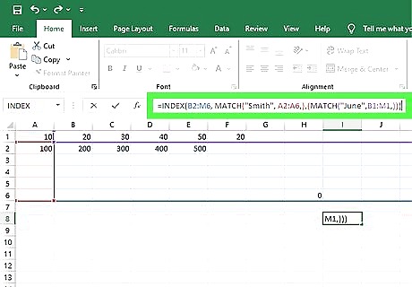
Fill in your variables. For example, imagine an Excel sheet listing employee names in column A and their monthly sales in columns B through M. If you wanted to find Smith's sales for June, you could write an INDEX MATCH function to find it. Your INDEX cell range would be the range of cells that include the sales numbers. In this example, if you had 5 employees and the first row was reserved for column headers, your INDEX cell range would be B2:M6. Your first MATCH function should be the row you are searching through. In this example, we are looking at a column of names, so a single name (Smith's) will be in a row. The lookup value should be Smith's name, and the lookup array should be the column the names are in, which is A1:A6 in this example. Your second MATCH function will be the column you're searching through. This column will intersect with the row specified in the earlier MATCH function, and the intersecting cell will be the returned value. In this example, we're looking at a row of months, so a single month (June) will be in a column. The lookup value should be June, and the lookup array should be the row that the names are in. In this example, that is B1:M1. Combine all of the parts. For the example set above, your final function should look like =INDEX(B2:M6, MATCH("Smith", A2:A6,),(MATCH("June",B1:M1,))). Whatever cell this function is written in will display Smith's sales for June. Replacing your lookup values can make this function even more dynamic. To the side of your Excel sheet, put Smith's name and the word June. Go back to your function and replace "Smith" with a reference to the cell in which you put Smith's name and replace "June" with a reference to the cell where you put the word June. This function can now be changed to look up the sales for any employee in the Excel sheet for any month by simply changing the values of the cells that say "Smith" and "June."
Multiple Criteria with Boolean Arrays
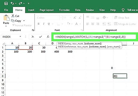
Use Boolean logic to create an INDEX MATCH function for multiple criteria. If you need to create a lookup that has values with multiple criteria, you will need to create an array with Boolean logic, which is a more advanced formula. The syntax for this function is =INDEX(range1,MATCH(1,(A1=range2)*(B1=range3),0)). If you have more criteria to search, you can add more to the array by adding (C1=range4)*(D1=range5), etc.

Fill in your variables. Imagine you have a 3 by 7 table that holds information about cakes you sell. The first column lists the flavors, the second column lists the sizes, and the third column lists the prices. Thus, each row lists each cake's flavor, size, and associated price. If you want to find out the price of a cake by just typing in the flavor and size, you can use an INDEX MATCH function with a Boolean array. Start by creating a key off to the side. Add a cell for a flavor name and a cell for size. These cells will be referenced in the Boolean array. In this example, we will put the flavor in F1 and the size in F2, with the price to be returned in F3. Your INDEX range1 should be your prices, since that's the information we're trying to return. In this example, the prices are in the cell range C2:C7. A1=range2 should be the first column you want to search. In this example, the first column we're searching for is flavor. The flavor is listed in F1, and our flavors are listed in A2:A7. So, the first part of your Boolean array will be (F1=A2:A7). B1=range3 should be the first column you want to search. In this example, the second column we're searching for is size. The size is in F2, and our flavors are in A2:A7. So, the second part of your Boolean array will be (F2=B2:B7).

Combine your arguments into one INDEX MATCH function. Your final function should look like =INDEX(C2:C7,MATCH(1,(F1=A2:A7)*(F2=B2:B7),0)) for the cell reference examples above. When entering a Boolean array, you must press Ctrl+Alt+↵ Enter for it to run. You can create sophisticated lookups if you combine two-way INDEX MATCH lookups with this Boolean array INDEX MATCH lookup. Instead of manually typing in the flavor and size into F1 and F2, you can create a separate customer table (on the same sheet) that lists each customer's name, the size of cake they ordered, and the flavor of cake they ordered, and then use this table to create two-way INDEX MATCH lookups that will automatically fill F1 and F2 with the cake flavor and size the customer ordered, which will then be pulled into the Boolean array INDEX MATCH lookup to lookup the price.


Comments
0 comment